HYBRID METHOD
Following from: Radiative transfer in coupled atmosphere and ocean systems: Monte Carlo method
To better solve the radiative transfer equations in specific situations, people have used hybrid radiative transfer models that combine the computational power of more than one of the radiative transfer methods introduced above. For example, Zhai et al. (2008a,b) reported a hybrid matrix operator-Monte Carlo (HMOMC) method that is optimized for simulations of the light field under dynamic ocean surfaces. Ota et al. (2010) reported a hybrid matrix formulation that uses both the discrete ordinate and matrix operator methods. In this article, we will only introduce the HMOMC method.
Almost all radiative transfer methods assume that the coupled atmosphere-ocean system is static. The air-sea interface is considered to be either flat or roughened, but is treated using the static Cox-Munk wave slope model, which gives reasonably good results for understanding the time-averaged light field. However, the real light field in a coupled atmosphere-ocean system (CAOS), especially that just beneath the air-sea interface, is highly dynamic and dominated by the instantaneous wavy ocean surface above it. To solve for the dynamic radiation field using conventional radiative transfer (RT) methods in this scenario, one has to run the complete RT model for each individual frame, which makes it highly inefficient and virtually impractical. Recently, as part of the effort in the Radiance in a Dynamic Ocean (RaDyO) project, a hybrid method (Zhai et al., 2008b) combining the power of both the matrix operator and Monte Carlo methods has been reported to make dynamic simulations practical.
The dynamic CAOS is inherently a 3D system since horizontal inhomogeneity in the light field is introduced by the instantaneous wave slope field. Therefore, the 1D matrix operator formalism has to be extented to 3D, where an impulse-response function is not only a function of the impulse and response directions ni and nr, but is also a function of the impulse and response positions ri and rr. It can be compactly written as a 16-dimensional matrix F(ρ(r),ρ(i)), where ρ = (r,n) denotes a combination of both the position and direction vectors. Each subset of this multidimensional matrix is in turn a 2D 4 × 4 Mueller matrix. The dynamic nature of the system introduces an extra temporal argument t, such that an impulse-response function becomes F(ρ(r),ρ(i);t). Keep in mind here that working on matrices implies that the angular and spatial dimensions are both discretized into grids. Specifically, the horizontal dimension has to be considered finite (unlike other methods that assume a semi-infinite plane-parallel system) with positions r being discretized grid points in the finite horizontal domain. Boundary conditions, such as simple periodic boundary conditions, are used to extend the finite computational domain to infinity.
Similar to the conventional matrix operator method, the hybrid method expresses the dynamic polarized underwater light field Id(ρ(d);t) as

|
(1) |
where d denotes the depth of the detector below the ocean surface, and D0d(ρ(d),ρ(0);t) is the effective detector response function that relates a detector response at a given ρ(d) to the incident light field at any ρ(0). The temporal variation in the light field is explicitly shown in Eq. (1). To describe D0d(ρ(d),ρ(0);t) in the matrix operator formalism, it is most convenient to partition the CAOS into three parts, namely, the atomsphere, the ocean surface, and the ocean along with its bottom. The top of the atmosphere, the bottom of the atmosphere/the top of the surface, the bottom of the surface/the top of the ocean, and the bottom of the ocean are labeled as levels 0, 1, 2, and 3, respectively in Fig. 1. The level of the underwater detector, d, is also shown. With this partition, D0d(ρ(d),ρ(0);t) in Eq. (1) can be expanded and compactly written as
|
(2) |
where only the first two orders of coupling terms are explicitly shown. Arguments ρ(r) and ρ(i) are suppressed for simplicity. These coupling terms are illustrated in Fig. 1 as well.
Figure 1. Partition of the CAOS into three parts, and the first two orders of coupling terms.
To design a more computationally efficient method for the light field immediately below the air-sea interface in a dynamic CAOS, note that the dynamic characteristics of the system are mainly carried by the surface layer, where the temporal variations can be much less than a second. Therefore, the impulse-response functions in this layer [such as T12(ρ(r),ρ(i);t) and R21(ρ(r),ρ(i);t)] have to be considered dynamic. On the other hand, the optical properties in the atmosphere and ocean parts are at most slowly varying on the order of minutes, if turbulence is not considered. Therefore, these two parts can be treated statically, and the corresponding impulse-response functions can be considered temporally independent; for example, T01(ρ(r),ρ(i)) and R01(ρ(r),ρ(i)). With these properties considered, Eq. (2) reduces to

|
(3) |
In the conventional matrix operator method, one has to first calculate the radiative transfer (i.e., the impulse-response functions) for infinitesimally thin layers, and then couple these functions to get it for the whole atmosphere/ocean system. In the HMOMC model, the whole atmosphere is treated as an integrated system, whose 3D impulse-response functions are precalculated from 3D Monte Carlo calculations (Zhai et al., 2008a). This applies to the whole ocean, including its bottom as well. These static atmospheric and oceanic impulse-response functions (for example, T01, T12, and D2d) are then coupled to those in the dynamic surface layer [for example, T12(t) and R21(t)], which are determined by Fresnel formulas. The coupling is done by a 3D expansion of the matrix operator method as previously mentioned to get the dynamic underwater light field. Using this coupling scheme, no computational efforts are wasted in unnecessary calculations of radiative transfer in the virtually static atmosphere and ocean parts at all instances in time. This makes it much more efficient than a conventional RT method (for example, a direct 3D Monte Carlo method) for the purpose of calculating the dynamic underwater light field just below the air-sea interface.
A dual-grid scheme reported by You et al. (2009) can be employed to further improve the computational efficiency of the HMOMC method. Notice that the wavelengths of typical gravity and capillary waves in real ocean surfaces are on the order of centimeters or even millimeters. To resolve these wave structures, one has to discretize the horizontal computational domain into very small grids, which makes the computation and the storage of necessary impulse-response functions prohibitively difficult. On the other hand, the optical properties of the atmosphere and ocean are usually horizontaly homogeneous on a much larger scale, and can be discretized into coarser grids. A grid size on the order of meters is sufficient for open waters, and can be smaller for relatively dyamic coastal waters. In the dual-grid scheme, the atmosphere and ocean parts are discretized into larger medium grids, while the ocean surface is discretized into smaller surface grids (Fig. 2). In this scheme, there are multiple surface grids that correspond to the same medium grid.

Figure 2. Discretizations of the computational domain in the single-grid scheme (a), and the dual-grid scheme (b) (adapted from You et al. 2009).
Special attention is needed to appropriately couple the medium and surface grids. For example, in the coupling term D2d · T12(t) · T01, the same medium impulse-response functions T01(ρ(r),ρ(i)) and D2d(ρ(r),ρ(i)) will be used for all surface grids that correspond to the same medium grid. This dual-grid scheme substantially reduces the required computational resources and satisfactorily keeps the accuracy of the computed light field. Figure 3 shows angular and spatial distributions of the downwelling radiance field as viewed by an array of nine detectors immediately beneath a dynamic ocean surface computed from the HMOMC method. The detectors are about 1.4 m away from each other. The horizontal inhomogeneity is obvious in Fig. 3. The temporal variation can be seen in the simulated “time series” of the radiance field (You et al., 2009).
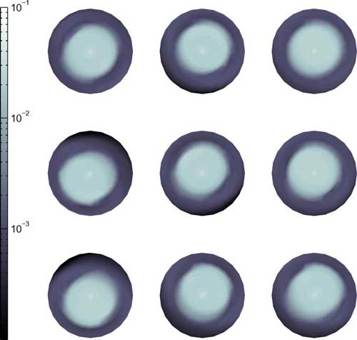
Figure 3. Simulated angular and spatial distributions of the radiance field immediately beneath a dynamic ocean surface (adapted from You et al., 2009).
A fast irradiance version of the HMOMC method (Fig. 4, You et al., 2010) has been developed to simulate the high-frequency temporal fluctuations in the downwelling irradiance beneath a dynamic ocean surface. Using this fast model, it is possible to simulate the temporal variations in the underwater downwelling irradiance Ed(t) to within several meters of the ocean surface with an extremely high sampling rate. In the simulated 10-min-long time series of Ed(t) with a sampling rate of 1 kHz, the probability densities of the normalized instantaneous downwelling irradiance Ed(t) /⟨Ed⟩ at various depths are consistent with their counterparts from field measurements made during the RaDyO Santa Barbara Channel experiment.

Figure 4. Simulated and measured probability density functions of the normalized downwelling irradiance at various depths (adapted from You et al. 2010).
REFERENCES
Ota, Y., Higurashi, A., Nakajima, T., and Yokota, T, Matrix formulations of radiative transfer including the polarization effect in a coupled atmosphere-ocean system, J. Quant. Spectr. Radiat. Transfer, vol. 111, pp. 878-894, 2010.
You, Y., Zhai, P.-W., Kattawar, G. W., and Yang, P., Polarized radiance fields under a dynamic ocean surface: a three-dimensional radiative transfer solution, Appl. Opt., vol. 48, no. 16, pp. 3019-3029, 2009.
You, Y., Stramski, D., Darecki, M., and Kattawar, G. W., Modeling of wave-induced irradiance fluctuations at near-surface depths in the ocean: a comparison with measurements, Appl. Opt., vol. 49, no. 6, pp. 1041-1053, 2010.
Zhai, P.-W., Kattawar, G. W., and Yang, P., Impulse response solution to the three-dimensional vector radiative transfer equation in atmosphere-ocean systems. I. Monte Carlo method, Appl. Opt., vol. 47, pp. 1037-1047, 2008a.
Zhai, P.-W., Kattawar, G. W., and Yang, P., Impulse response solution to the three-dimensional vector radiative transfer equation in atmosphere-ocean systems. II. The hybrid matrix operator-Monte Carlo method, Appl. Opt., vol. 47, pp. 1063-1071, 2008b.
References
- Ota, Y., Higurashi, A., Nakajima, T., and Yokota, T, Matrix formulations of radiative transfer including the polarization effect in a coupled atmosphere-ocean system, J. Quant. Spectr. Radiat. Transfer, vol. 111, pp. 878-894, 2010.
- You, Y., Zhai, P.-W., Kattawar, G. W., and Yang, P., Polarized radiance fields under a dynamic ocean surface: a three-dimensional radiative transfer solution, Appl. Opt., vol. 48, no. 16, pp. 3019-3029, 2009.
- You, Y., Stramski, D., Darecki, M., and Kattawar, G. W., Modeling of wave-induced irradiance fluctuations at near-surface depths in the ocean: a comparison with measurements, Appl. Opt., vol. 49, no. 6, pp. 1041-1053, 2010.
- Zhai, P.-W., Kattawar, G. W., and Yang, P., Impulse response solution to the three-dimensional vector radiative transfer equation in atmosphere-ocean systems. I. Monte Carlo method, Appl. Opt., vol. 47, pp. 1037-1047, 2008a.
- Zhai, P.-W., Kattawar, G. W., and Yang, P., Impulse response solution to the three-dimensional vector radiative transfer equation in atmosphere-ocean systems. II. The hybrid matrix operator-Monte Carlo method, Appl. Opt., vol. 47, pp. 1063-1071, 2008b.