RADIATIVE TRANSFER IN COUPLED ATMOSPHERE AND OCEAN SYSTEMS: THE SUCCESSIVE ORDER OF SCATTERING METHOD
Following from: Radiative transfer for coupled atmosphere and ocean systems: the discrete ordinate method
Leading to: Radiative transfer in coupled atmosphere and ocean systems: the discrete ordinate method
The successive order of scattering (SOS) method is a very useful method because it is based on physical intuition and is easy to understand. Lenoble (1985) contains a large list of references. The method remains an active research area since then (Myneni et al., 1987; Lenoble, 1993). Techniques have been developed to make SOS more efficient (Min and Duan, 2004; Duan and Min, 2005). It is also easy to include polarization with the SOS method (Lenoble et al., 2007). Particularly, it is used to solve the RTE in the coupled atmosphere and ocean systems (AOS) (Chami et al., 2001; Kotchenova et al., 2006; Kotchenova and Vermote, 2007; Zhai et al., 2009, 2010; Tanaka, 2010). There are also many other publications on the SOS method (e.g., Greenwald et al., 2005; Suzuki et al., 2007).
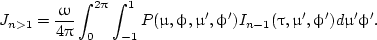
The starting point is to decompose the radiance into contributions from different scattering order In,

|
(1) |
where N is the maximum order of scattering determined by the condition of res ≈ 0. Note that I0 = Fsδ(μ-μ0)δ(ϕ-ϕ0) is the direct solar light, and Fs is the solar irradiance perpendicular to the solar beam. Substitute Eq. (1) into Eqs. (11) and (12) of Zhai and Hu (2011), and one gets

|
(2) |

|
(3) |
where

|
(4) |
|
(5) |
The first source term in Eq. (4) is due the direct solar irradiance Fsδ(μ-μ0)δ(ϕ-ϕ0) incident into the system at τ = τl. The angle between the solar incident angle and the zenith is θ0 and μ0 = cos(θ0) < 0. Equations (1)-(5) are equivalent to Eqs. (10)-(12) of Zhai and Hu (2011), which can be shown by substituting Eqs. (4) and (5) into Eqs. (2) and (3) and summing up according to Eq. (1). Note that Eq. (1) represents the diffuse radiance field, in which the known direct solar light has been excluded for convenience.
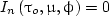
Using some physical intuition, the radiance field I1from single scattering is obtained by substituting J1 into Eqs.(2) and (3). In(τl,μ,ϕ) = 0 and In(τu,μ,ϕ) = 0 if no dielectric interface is present. The higher-order contributions In > 1 can be found by the use of Eq. (5) and Eqs. (2) and (3), successively. This is the essence of the SOS method. The angular integrations involved in Eq. (5) may be evaluated by numerical methods, for instance, the Gaussian quadrature method (Press et al., 2007). Note that the 2D integration is cumbersome, and the accuracy is often not promising. A common practice is to expand the radiance field and phase function into Fourier series in ϕ. The RTE is then decomposed into equations depending on Fourier order number m. The equations with different m are completely decoupled, and can be solved separately (Lenoble et al., 2007). Both efficiency and accuracy can be improved in this way. The optical depth integration in Eqs. (2) and (3) maybe evaluated by a similar quadrature method or the exponential-linear in depth approximation for efficiency (Kylling and Stamnes, 1992). The SOS can also be used to solve the RTE including polarization (Chami et al., 2001; Lenoble et al., 2007; Zhai et al., 2009, 2010). We refer the readers to the references for these more advanced topics.
The above description of the SOS method does not include an interface across which the refractive index changes. For the AOS that includes such an interface, the boundary conditions described in Zhai and Hu (2011) need to be considered. For convenience, hereafter, we denote that the atmospheric optical depth is bounded by 0 < τ < τa and the ocean optical depth by τo < τa < τo*, respectively; and τo = τa + ζ, where ζ is an infinitesimal in our model. The application of the SOS method to the AOS with a flat ocean surface is relatively easy and will be treated first.
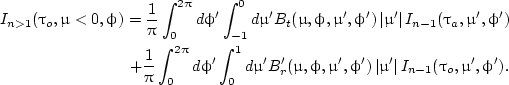
Figure 2 in Zhai and Hu (2011) shows a schematic picture of the AOS with a flat ocean surface. A solar source light is incident into the AOS, and the incident angle of the direct solar light is θi < π < θo. The light will be reflected and refracted (transmitted) by the ocean interface. The reflection angle θr is equal to the incident angle θi, and the transmission angle θt = θ'0 is determined by Snell’s law, i.e., sinθi = nwsinθ'0, where nw is the refractive index of water. The direct solar and reflected light can induce the second order diffuse light in the atmosphere. The light transmitted into the ocean can induce second-order diffuse light in the ocean as well. Equations (2) and (3) are still applicable to this situation with the understanding that τl = 0 and τu = τa for atmosphere, and τl = τo and τu = τo* for ocean. Also, In(τl,μ,ϕ) and In(τu,μ,ϕ) have to satisfy the interaction principles Eqs. (14) in (Zhai and Hu 2011). In addition, the first-order source function [Eq. (4)] needs to be updated as follows:

|
(6) |

|
(7) |
We have made the phase function a function of optical depth to make it applicable to more general cases. Equation (5) is still valid with the understanding that P is dependent on the optical depth. In the atmosphere, τ < τa, the extra source term, represents the direct solar light reflected by the ocean interface. In the ocean, τ > τo, the first term on the right-hand side, is the direct solar light transmitted through the interface. In Eq. (7), μ'0 = cos(θ'0). The factor μ0/μ'0 is to take into account the projected area difference between the incident and refracted rays. Ta and To are the temperatures of the atmosphere and ocean, respectively. The boundary conditions are (Zhai et al., 2009)
|
(8a) |
|
(8b) |

|
(8c) |

|
(8d) |

|
(8e) |

|
(8f) |
The reflection of the ocean bottom has been assumed to be zero. μ' = cos(θ') and sinθ = nwsinθ' in Eqs. (8c) and (8d). The physical interpretations of Eqs. (8) are as follows:
- The radiance boundary condition at the top of the atmosphere (TOA) are always zero. Note that the external solar irradiance source has been included in the source function [Eq. (6)]. Also, this does not mean that the final radiance field at that TOA will be zero. Generally, the upwelling radiance will not be zero as a result of multiple scattering shown in Eqs. (2) and (3).
- At the bottom of the atmosphere, the first-order radiance boundary condition is zero since the solar glint has been included in the source function [Eq. (6)]. For higher-order scattering, the boundary condition is the interaction principles for the flat interface.
- At the top of the ocean, the first-order scattering contribution is included in Eq. (7) so that the downwelling radiance is zero. Again, the interaction principles guide the higher-order scattering radiance.
- The ocean bottom is assumed to be totally absorbing (no reflection).
For the case of a rough ocean surface, the BRDF and BTDF will take the places of reflection and transmission coefficients r and t. We still use Eqs. (2) and (3) for our fundamental equations for both the atmosphere and ocean. The source functions and boundary conditions are modified as follows:

|
(9a) |

|
(9b) |

|
(9c) |

|
(9d) |

|
(9e) |
|
(9f) |
Next, we will calculate the radiance field for an ideal AOS to show some special characteristics of ocean optics. Both the atmosphere and ocean are Rayleigh scattering media with no absorption, i.e., the single-scattering albedos are the optical depths of the atmosphere and ocean are 0.1 and 1, respectively. The ocean surface is flat, and the refractive index is nw = 1.34. The radiance field is calculated by both the SOS (Zhai et al., 2010) and Monte Carlo (MC) methods (Kattawar and You, 2011; Zhai et al., 2008). The light source is solar light with the solar zenith angle θ0 = 120 deg. The solar irradiance is Fs = π. The thermal source is ignored. Two detector positions are selected to show results; one is just above the ocean surface, and the other is just below the ocean surface. Figure 1 shows the diffuse radiance just above the ocean surface calculated by the two methods. Four azimuth planes ϕ - ϕ0 = 0, 60, 120, 180 deg are shown, where ϕ and ϕ0 are the azimuth angles for the viewing and solar source directions, respectively. The radiance is shown as a function of viewing zenith angle θ. The zenith angle (θ < 90) means the radiance is upwelling and vice versa. Figure 1 shows excellent agreement between the two methods. The downwelling radiances (θ > 90) are smoother than the upwelling radiances for all four azimuth planes. The downwelling radiances are resultant of Rayleigh multiple scattering, which is supposed to be smooth. On the other hand, the upwelling radiances include two parts, i.e., the radiances from specular reflection and those transmitted from underwater (interaction principle, see Zhai and Hu, 2011). The reflection and transmission coefficients of a typical water interface are relatively flat for small incident angles, but changes rapidly for incident angles that are >60 deg (Kattawar and Adam, 1989). This is the reason of the relatively larger slope of the radiance field for upwelling radiances.

Figure 1. Radiance just above the ocean surface for a coupled atmosphere and ocean system; both the atmosphere and ocean media are conservative Rayleigh; the optical depths of the atmosphere and ocean are 0.1 and 1.0, respectively.
Figure 2 shows the radiance field just below the ocean surface for the same case. The most prominent feature is the symmetry between the downwelling and upwelling radiances around θ = 90o. This is because the total reflection of light by a water surface if light is incident from the water and the incident angle is larger than the critical angle θc. The critical angle θc is determined by nwsinθc = sin90 deg = 1, which leads to θc = 48.2682 deg for nw = 1.34. Also, the radiances transmitted from the atmosphere will be all confined within θ > π - θc, which is called the Fresnel cone in ocean optics. Therefore, it is understood that the downwelling radiances for θ < π - θc are due to the total reflection of upwelling radiances without any contribution from the atmosphere transmission. On the other hand, the radiances within the Fresnel cone θ > π - θc contain both the atmospheric transmission and oceanic reflection. Discontinuity is observed at π - θc for all radiances due to this phenomenon.

Figure 2. Radiance just below the ocean surface for the same case as Fig. 1; the legend is also the same as Fig. 1.
The SOS method for the AOS has wide applications in ocean color remote sensing. Chami and Platel (2007) used their ordre sucessifs ocean atmosphere (OSOA) radiative transfer model based on the SOS method to train a neural network algorithm that retrieves the inherent optical properties of ocean water. In ocean color remote sensing, one primary task is to remove the atmospheric radiance from the total radiance at the top of the atmosphere to get the water leaving radiance (contribution from under the water). This procedure is called the atmospheric correction. The 6S model based on the SOS method is used to calculate the lookup tables used in the atmospheric correction for the moderate resolution imaging spectroradiometer (MODIS) satellite instrument (Kotchenova et al.. 2006). Zhai et al. (2010b) have studied the decoupling error in the atmosphere correction procedure using their SOS model for the AOS.
REFERENCES
Chami, M., Santer, R., and Dilligeard, E., Radiative Transfer Model for the Computation of Radiance and Polarization in an Ocean-Atmosphere System: Polarization Properties of Suspended Matter for Remote Sensing, Appl. Opt., vol. 40, pp. 2398-2416, 2001.
Chami, M. and Platel, M. D., Sensitivity of the Retrieval of the Inherent Optical Properties of Marine Particles in Coastal Waters to the Directional Variations and the Polarization of the Reflectance, J. Geophys. Res., vol. 112, C05037, 2007.
Duan, M. and Min, Q., A Semi-Analytic Technique to Speed Up Successive Order of Scattering Model for Optically Thick Media, J. Quant. Spectrosc. Radiat. Transfer, vol. 95, pp. 21-32, 2005.
Greenwald, T., Bennartz, R., O'Dell, C., and Heidinger, A., Fast Computation of Microwave Radiances for Data Assimilation Using the Successive Order of Scattering Method, J. Appl. Meteorol., vol. 44, pp. 960-966, 2005.
Kattawar, G. W. and Adams, C. N., Stokes Vector Calculations of the Submarine Light Field in an Atmosphere-Ocean with Scattering According to a Rayleigh Phase Matrix: Effect of Interface Refractive Index on Radiance and Polarization, Limnol. Oceanog., vol. 34, pp. 1453-1472, 1989.
Kattawar, G. W. and You, Y., Radiative Transfer for Coupled Atmosphere and Ocean Systems: The Monte Carlo Method, Thermopedia, 2011.
Kotchenova, S. Y., Vermote, E. F., Matarrese, R., and Klemm, F. J., Jr., Validation of a Vector Version of the 6S Radiative Transfer Code for Atmospheric Correction of Satellite Data. Part I: Path Radiance, Appl. Opt., vol. 45, pp. 6762-6774, 2006.
Kotchenova, S. Y. and Vermote, E. F., Validation of a Vector Version of the 6S Radiative Transfer Code for Atmospheric Correction of Satellite Data. Part II. Homogeneous Lambertian and Anisotropic Surfaces, Appl. Opt., vol. 46, pp. 4455-4464, 2007.
Kylling, A. and Stamnes, K., Efficient yet Accurate Solution of the Linear Transport Equation in the Presence of Internal Sources: The Exponential-Linear in Depth Approximation, J. Comput. Phys., vol. 102, pp. 265-276, 1992.
Lenoble, J., Atmospheric Radiative Transfer, A. Deepak Publishing, Hampton, VA, 1993.
Lenoble, J., Radiative Transfer in Scattering and Absorbing Atmospheres: Standard Computational Procedures, A. Deepak Publishing, Hampton, VA, 1985.
Lenoble, J, Herman, M, Deuzé, J. L., Lafrance, B., Santer, R., and Tanré, D., A Successive Order of Scattering Code for Solving the Vector Equation of Transfer in the Earth’s Atmosphere with Aerosols, J. Quant. Spectrosc. Radiat. Transfer, vol. 107, pp. 479-507, 2007.
Min, Q. and Duan, M., A Successive Order of Scattering Model for Solving Vector Radiative Transfer in the Atmosphere, J. Quant. Spectrosc. Radiat. Transfer, vol. 87, pp. 243-259, 2004.
Myneni, R. B., Asrar, G., and Kanemasu, E. T., Light Scattering in Plant Canopies: The Method of Successive Orders of Scattering Approximations (SOSA), Agri. Meteorol., vol. 39, pp. 1-12, 1987.
Press, W. H., Teukolsky, S. A., Vetterling, W. T., and Flannery, B. P., Numerical Recipes:The Art of Scientific Computing, 3rd ed., Cambridge, New York, 2007.
Suzuki, T., Nakajima, T., and Tanaka, M., Scaling Algorithms for the Calculation of Solar Radiative Fluxes, J. Quant. Spectrosc. Radiat. Transfer, vol. 107, pp. 458-469, 2007.
Tanaka, A., Numerical Model Based on Successive Order of Scattering Method for Computing Radiance Distribution of Underwater Light Fields, Opt. Express, vol. 18, pp. 10127-10136, 2010.
Zhai, P., Kattawar, G. W., and Yang, P., Impulse Response Solution to the Three-Dimensional Vector Radiative Transfer Equation in Atmosphere-Ocean Systems, I. Monte Carlo Method, Appl. Opt., vol. 47, pp. 1037-1047, 2008.
Zhai, P., Hu, Y., Trepte, C. R., and Lucker, P. L., A Vector Radiative Transfer Model for Coupled Atmosphere and Ocean Systems Based on Successive Order of Scattering Method, Opt. Express, vol. 17, pp. 2057-2079, 2009.
Zhai, P., Hu, Y., Trepte, C. R., and Lucker, P. L., A vector radiative transfer model for coupled atmosphere and ocean systems with a rough interface, J. Quant. Spectrosc. Radiat. Transfer, vol. 111, pp. 1025-1040, 2010a.
Zhai, P., Hu, Y., Trepte, C. R., Lucker, P. L., and Josset, D. B., Decoupling Error for the Atmospheric Correction in Ocean Color Remote Sensing Algorithms, J. Quant. Spectrosc. Radiat. Transfer, 111, no. 12-13, pp. 1958-1963, 2010b.
Zhai, P. and Hu, Y., Radiative Transfer for Coupled Atmosphere and Ocean Systems: Overview, Thermopedia, 2011.
References
- Chami, M., Santer, R., and Dilligeard, E., Radiative Transfer Model for the Computation of Radiance and Polarization in an Ocean-Atmosphere System: Polarization Properties of Suspended Matter for Remote Sensing, Appl. Opt., vol. 40, pp. 2398-2416, 2001.
- Chami, M. and Platel, M. D., Sensitivity of the Retrieval of the Inherent Optical Properties of Marine Particles in Coastal Waters to the Directional Variations and the Polarization of the Reflectance, J. Geophys. Res., vol. 112, C05037, 2007.
- Duan, M. and Min, Q., A Semi-Analytic Technique to Speed Up Successive Order of Scattering Model for Optically Thick Media, J. Quant. Spectrosc. Radiat. Transfer, vol. 95, pp. 21-32, 2005.
- Greenwald, T., Bennartz, R., O'Dell, C., and Heidinger, A., Fast Computation of Microwave Radiances for Data Assimilation Using the Successive Order of Scattering Method, J. Appl. Meteorol., vol. 44, pp. 960-966, 2005.
- Kattawar, G. W. and Adams, C. N., Stokes Vector Calculations of the Submarine Light Field in an Atmosphere-Ocean with Scattering According to a Rayleigh Phase Matrix: Effect of Interface Refractive Index on Radiance and Polarization, Limnol. Oceanog., vol. 34, pp. 1453-1472, 1989.
- Kattawar, G. W. and You, Y., Radiative Transfer for Coupled Atmosphere and Ocean Systems: The Monte Carlo Method, Thermopedia, 2011.
- Kotchenova, S. Y., Vermote, E. F., Matarrese, R., and Klemm, F. J., Jr., Validation of a Vector Version of the 6S Radiative Transfer Code for Atmospheric Correction of Satellite Data. Part I: Path Radiance, Appl. Opt., vol. 45, pp. 6762-6774, 2006.
- Kotchenova, S. Y. and Vermote, E. F., Validation of a Vector Version of the 6S Radiative Transfer Code for Atmospheric Correction of Satellite Data. Part II. Homogeneous Lambertian and Anisotropic Surfaces, Appl. Opt., vol. 46, pp. 4455-4464, 2007.
- Kylling, A. and Stamnes, K., Efficient yet Accurate Solution of the Linear Transport Equation in the Presence of Internal Sources: The Exponential-Linear in Depth Approximation, J. Comput. Phys., vol. 102, pp. 265-276, 1992.
- Lenoble, J., Atmospheric Radiative Transfer, A. Deepak Publishing, Hampton, VA, 1993.
- Lenoble, J., Radiative Transfer in Scattering and Absorbing Atmospheres: Standard Computational Procedures, A. Deepak Publishing, Hampton, VA, 1985.
- Lenoble, J, Herman, M, Deuzé, J. L., Lafrance, B., Santer, R., and Tanré, D., A Successive Order of Scattering Code for Solving the Vector Equation of Transfer in the Earth’s Atmosphere with Aerosols, J. Quant. Spectrosc. Radiat. Transfer, vol. 107, pp. 479-507, 2007.
- Min, Q. and Duan, M., A Successive Order of Scattering Model for Solving Vector Radiative Transfer in the Atmosphere, J. Quant. Spectrosc. Radiat. Transfer, vol. 87, pp. 243-259, 2004.
- Myneni, R. B., Asrar, G., and Kanemasu, E. T., Light Scattering in Plant Canopies: The Method of Successive Orders of Scattering Approximations (SOSA), Agri. Meteorol., vol. 39, pp. 1-12, 1987.
- Press, W. H., Teukolsky, S. A., Vetterling, W. T., and Flannery, B. P., Numerical Recipes:The Art of Scientific Computing, 3rd ed., Cambridge, New York, 2007.
- Suzuki, T., Nakajima, T., and Tanaka, M., Scaling Algorithms for the Calculation of Solar Radiative Fluxes, J. Quant. Spectrosc. Radiat. Transfer, vol. 107, pp. 458-469, 2007.
- Tanaka, A., Numerical Model Based on Successive Order of Scattering Method for Computing Radiance Distribution of Underwater Light Fields, Opt. Express, vol. 18, pp. 10127-10136, 2010.
- Zhai, P., Kattawar, G. W., and Yang, P., Impulse Response Solution to the Three-Dimensional Vector Radiative Transfer Equation in Atmosphere-Ocean Systems, I. Monte Carlo Method, Appl. Opt., vol. 47, pp. 1037-1047, 2008.
- Zhai, P., Hu, Y., Trepte, C. R., and Lucker, P. L., A Vector Radiative Transfer Model for Coupled Atmosphere and Ocean Systems Based on Successive Order of Scattering Method, Opt. Express, vol. 17, pp. 2057-2079, 2009.
- Zhai, P., Hu, Y., Trepte, C. R., and Lucker, P. L., A vector radiative transfer model for coupled atmosphere and ocean systems with a rough interface, J. Quant. Spectrosc. Radiat. Transfer, vol. 111, pp. 1025-1040, 2010a.
- Zhai, P., Hu, Y., Trepte, C. R., Lucker, P. L., and Josset, D. B., Decoupling Error for the Atmospheric Correction in Ocean Color Remote Sensing Algorithms, J. Quant. Spectrosc. Radiat. Transfer, 111, no. 12-13, pp. 1958-1963, 2010b.
- Zhai, P. and Hu, Y., Radiative Transfer for Coupled Atmosphere and Ocean Systems: Overview, Thermopedia, 2011.